Part 1 Principles
1. Fluorescence microscope
2. Filterset in FL-Mic
3. How concocal differs?
4. What is confocal?
5. Resolution in confocal
6. Optical sectioning
7. Confocal image formation
    and time resolution
8. SNR in confocal
9. Variations of confocal
      microscope
10. Special features from
     Leica sp2 confocal
Part 2 Application
1. Introduction
2. Tomographic view
    (Microscopical CT)
3. Three-D reconstruction
4. Thick specimen
5. Physiological study
6. Fluorescence detecting
       General consideration
       Multi-channel detecting
       Background  correction
       Cross-talk correction
            Cross excitation
            Cross emission
            Unwanted FRET

Part 3 Operation and
             Optimization
 1. Getting started
 2. Settings in detail
      Laser line selection
      Laser intensity and 
         AOTF control
      Beam splitter
      PMT gain and offset 
      Scan speed
      Scan format, Zoom
        and Resolution
     Frame average, and
         Frame accumulation
     Pinhole and Z-resolution
     Emission collecting rang
        and Sequential scan

When Do you need confocal?
FAQ
Are you abusing confocal?

Confocal Microscopy tutorial

Part 3 operation, optimization of Leica SP2 LSCM

1. Getting started: Brief Step-by-step guide (PDF file)

Leica SP2 confocal microscope is controlled via software LCS (Leica Confocal Software). The latest version is V2.5. Bellowing is a brief step-by-step guide to help new users get started smoothly. For detailed description about choosing related parameters, please refer to corresponding section in Part 3 of this guide, Operation and Optimization: Settings in detail.

1. Check your specimen under conventional fluorescent microscope, confirm the staining, and make a plan in advance on which laser or how many lasers you are going to use before you go to confocal microscope.

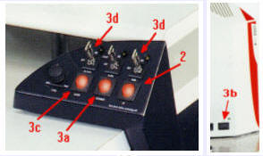
4. Turn on laser lines of your choice:
       Figure out which laser line or lines you are going to use before turning all of the lasers on.    
       Beware: each turn-on of laser costs life-time of the laser and is expensive.

• If you need 458/476/488/514 nm line, turn on Argon Laser:
  First, Argon Laser Fan (3c) on. without cooling fan, Argon laser will not work.
  After fan on, turn on Argon laser Power key (3d)-left.
• If you need 633 nm line, turn on He-Ne laser 633 by Power key (3d)-right. This laser does not need cooling fan.
• If you need 568 line, turn on  krypton laser 568 in a separate box on the floor.
  Same as Argon laser, Kr 568 has cooling fan button and its power key.

5. Turn on HBO mercury arc lamp on the granite table which is for conventional FL Microscopy.

6. Log in into your WinNT account with password.

7. Click Leica Confocal Software icon, wait for Initialization of Hardware  Note: Scanner 3a and microscope controller 3b must be on at least 30 sec before launching the program. Otherwise, the initialization will fail and it takes extra long time to end an unsuccessful initialization.

LCS has several function modules. The default module at start is Acquisition module.
The user interface of Acquisition Module looks like  the screen-shot below:

8.  Click Beam icon    This launch a parameter setting panel. Drag it to the center of the window.  The screen shot  looks like below:

9. you need choose a field of view under convention microscope before scanning. Click and press microscope control icon MicCtrl, choose visual from the pull-down menu.

Look at  microscope stand front panel, be sure Shutter light is off.
Put your slide upside down on microscope stage. For Objectives from 40 x on, use oil.

On the left side of microscope, there are two buttons for changing objectives. Objectives can also be changed from LSC software by Obj icon.

Note: to toggle between oil and dry Obj, you have to press simultaneously two arrow keys at same time on the front panel of the microscope stand, or use Obj icon and confirm the change when being asked.
On the right side of the microscope stand, there are two buttons for fast focus up and down adjusting in addition to the focus knob.

Choose filter-set for conventional fluorescence microscope, 3 filter-set available:
I3 for blue excitation, green emission (FITC, Alexa 488, etc.),
N2.1 for green excitation, red emission (Rhodamine, etc.).
Y5 for red Excitation, long red emission (CY5, Alexa 633, etc.).

Click MicCtrl again, choose Scan this time to switch back to confocal mode.

10. In  LCS  window, click one of the pre-settings from the list for different fluorescent dyes. The upper part of the list under Leica is protected from being changed. The lower part of the list under User holds all user modified and saved settings

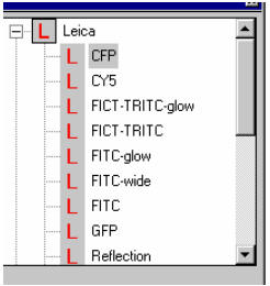By a single click on a pre-setting, you get all ten basic acquisition related parameters done, including laser, beam splitter, PMT and spectro-detecting range, LUT for PMT, etc. You can later modify them.

11. Set other six scan related parameters: scan Mode; Scan Speed; Scan Format; Pinhole size, Zoom factor and image Average respectively.
If this is the first scan after you launch the program, there are default values for these parameters, which usually you don't need change before scanning. These values are:

• Scan mode: xyz
• Scan speed: 400 Hz
• Scan format: 512 x 512
• Pinhole: 1 Airy unit
• Zoom factor: 1 x
• Image average: 1

If this is the later scan after specimen or field change, check these parameters and be sure return some of these values, especially zoom factor to 1 x, average to 1.

12. Click Continuous to begin scanning, while in scan, adjust other four in-line parameters: gain, offset of a given detecting channel to get optimal signal intensity, adjust Z-level to get a slice showing the specific structure of your interesting. These three parameters are the key players when you get a black image screen. Pinhole can also be adjusted to value other than 1 airy unit if desired.

All these four can be changed through a 7-knob-Control-Box.
The function of each knob can be defined at your will. The saved knob definition can be loaded from icon:

 13. The image will appear on image viewer at the right-side monitor. You can toggle image display mode among single channel, tiled (two or more channels), OVL overlay, Gallery, or play series. This can be done by clicking respective icon on the vertical tool bar on the left side of the image viewer window.

14. Scale bar, grids and coordinates can be superimposed on the image by checking scale, grids or coordinates box in the Function Overview panel on the lower-left side panel of the LCS main window below Experiment overview. please note, like color overlay, these overlaid marker are not saved by default, Export has to be used to fix these markers on image. See more at item 18: Data saved.

15. If you are interested in a specific region or cell rather than the whole field, you can make a region of interesting, scan only on that ROI by using Zoom In

16. If you are satisfied with the result, stop continuous scan. Usually, it is difficult or unnecessary to get a clear background  simply by adjusting gain and offset alone at the cost of signal intensity. Instead, you can tolerate some background noise to maintain reasonable intensity and use image average to improve SNR and quality of your image. 4-8 times average works for most cases.

17. Click Single Scan or Series scan (if applicable) to get the final data acquired..

18. Save and manipulating acquired data files:
It is better to understand some details about how LCS handle acquired data.

Experiment overview at upper-left side panel of the LCS main window is an important area for data file handling.
Please pay close attention to it during data acquisition.

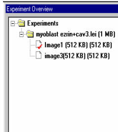
Multiple experiment overview windows can be opened by File/New or Save As command. Each experiment is represented by a folder icon and a *.lei name, and each has a  image viewer.

But all windows consume memory and lead to diminished computer resource. Delete Experiment from the experiments list  (the same thing as close image viewer window on the right-side monitor) removes data from memory, but not from disk if you have saved them already.

19. Data saved by LCS:
The saved data on hard disk are organized by experiments, i.e., the *.lei entries. Each entry is saved as a separate folder with TIF color image files for all detecting channel you have used. The image overlay of different channels or overlay of scale bar and grids on top of image, however, are not saved by default. To save them, you have to select them by right-mouse-click, choose "Export, Export selection" from the pop-up context menu. This will add an extra color image entry under the experiment overview panel, then they can be saved.
The color overlay or scale bar superimposing can be done later at any time if you re-load the original data into LCS program, providing the *.lei file remain untouched.

Saved together with TIF image files, the *.lei file is an important file which holds information of your confocal session and make the data active to LCS program as if you have just acquired them. Keep them within the folder if you want re-load and re-play or modify the image within LCS program.

20. File naming convention: When you click save, you will be prompted to enter a name. Please bear in mind: what you enter here is not a single file name, instead, it is the folder name for the experiment and it is also the first common part of file name for all images under the same .lei entry. After the first part, there are image-name, series number, channel number, TIF extension. All these can make very long file name if not named carefully. So, the first part doesn't need to be specific, just use a category name and as short as possible. After the experiment is saved, modify the second part "image-xx" to a short specific name. Other parts can not be modified. Long file name will be truncated if viewed under  Mac OS before OS X.

21. After confirm the saved files on the hard disk, you can turn off the system in a reversed order as you turn it on.

• Quit Leica control software.
• Turn off HBO mercury lamp, Turn off scanner.
• Turn off all laser keys. Don’t turn off Fan at this moment!. Let them running at least five minutes after the laser key off. Don’t forget Kr laser on the floor.
  Clean microscope objectives and stage, make working log during the 5 min time.
• Finally, turn off Leica microscope controller, turn off fans.
• Turn off PC.

This is just a quick flow-chart. Personal guide on advanced function can be obtained on request.