Part 1 Principles
1. Fluorescence microscope
2. Filterset in FL-Mic
3. How concocal differs?
4. What is confocal?
5. Resolution in confocal
6. Optical sectioning
7. Confocal image formation
    and time resolution
8. SNR in confocal
9. Variations of confocal
      microscope
10. Special features from
     Leica sp2 confocal
Part 2 Application
1. Introduction
2. Tomographic view
    (Microscopical CT)
3. Three-D reconstruction
4. Thick specimen
5. Physiological study
6. Fluorescence detecting
       General consideration
       Multi-channel detecting
       Background  correction
       Cross-talk correction
            Cross excitation
            Cross emission
            Unwanted FRET

Part 3 Operation and
             Optimization
 1. Getting started
 2. Settings in detail
      Laser line selection
      Laser intensity and 
         AOTF control
      Beam splitter
      PMT gain and offset 
      Scan speed
      Scan format, Zoom
        and Resolution
     Frame average, and
         Frame accumulation
     Pinhole and Z-resolution
     Emission collecting rang
        and Sequential scan

When Do you need confocal?
FAQ
Are you abusing confocal?

Confocal Microscopy tutorial

Part 1 Principles of Confocal microscopy

6. optical sectioning in confocal microscopy

     How does confocal microscope make optica sectioning?

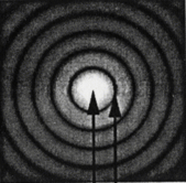
Point Spread Function (PSF) and confocal effect

As we mentioned before, in a confocal system there are two pinholes: A illumination pinhole for point light source and a detecting pinhole to get rid of out-of-focus image. Thus there are two point spread function: PSFs for source light which describes the distribution of point light in specimen plane and PSFd for detecting light which describes the distribution of point light image on the detecting plane. Since they two are independent events, mathematically, the probability of two independent events is the product of that two probabilities.

So, the total PSF of the confocal system is defined as PSFcf = PSFs x PSFd.

Since probability is a always smaller than 1, the product of two probability is always smaller than its individual probability. 
In case of Airy disk: at  the central peak: 0.84 x 0.84 = 0.656
while for the third ring: it is 0.06 x 0.06 = 0.0036.
For a spot with 0.01 original intensity, the final intensity will be only 0.0001, thus below the detecting threshold and is ignored by the detector.

These number tell us that, for out-of-focus image, the farther a point is off the focal plane, the more dramatic the signal decreases. It gets so weak at some distance that it is well below the detecting threshold of the system then is no longer detectable. This is the fundamental mechanism of confocal effect or optical sectioning.

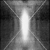
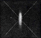
Figures below show this effect graphically.

Axial: without pinhole         Axial: with pinhole       Lateral: without pinhole  Lateral: with pinhole

So, the confocal effect and optical sectioning work at the cost of great reduction of total detecting volume.
For example, at 488 nm excitation:
the thickness of optical section, by Formula 3: 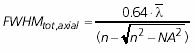, is about 500 nm. For a cultured cell at 12 µ, this is less than 1/20 of its total volume.

Side effects of reduced detecting volume

• Deteriorated signal to background ratio SNR

The general reduction of detecting volume has much more effect on signal than on background noise since some types of background noise are constant or affected less by confocal effect. That means the SNR (signal to noise ratio) and image quality become worse as signal decrease,
Formula 4: 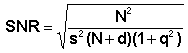describes this relationship. N is number of photons which has squared effect on SNR.

This makes confocal microscope very vulnerable to weak signal. The reduction will make signal weaken to a level similar to or just a little bit higher than background and can not be enhanced by manipulating gain or threshold on PMT. In this case, the image quality is even worse than what can be taken from a digital camera based conventional fluorescence microscope, the resolution gain and all advantages over conventional microscopy is lost here. You even don't have usable data at all.

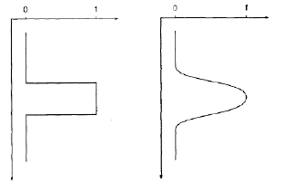It is also worth noting that the optical section is not a neat section like cut by a microtome. It does not begin and end abruptly in acute angle as in mechnical cutting, instead, it looks like a figure shown on the left.
Pinhole makes optical section possible. Pinhole size also determine the thickness of the optical section. Theoretically, the thickness of the optical section reach the thinnest when the pinhole size is zero or close to infinite small. At this point, it equals to the axial resolution of the lens as predicted by the formula listed above.

But pinhole can not be zero or infinite small, it must has a physical size for image to be detected. So, the optical section is always thicker than Z-resolution of the lens.  Formula 5 below 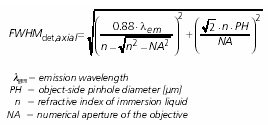shows the influence of pinhole size on section thickness when pinhole is > 1 AU.

When pinhole size is between 0.25-1 AU, the above Formula 3 for axial resolution can be used to approximate the optical section thickness by using value between 0.64 and 0.88 to replace 0.64 in the formula. For pinhole = 1 AU, 0.88 is used for calculation. This formula requires physical size of pinhole in use and is much more complicated for calculation. For estimating, one can use the axial Resolution. But bear in mind the section is thicker than predicted from axial resolution, or simply taking, it is roughly double size of the lateral resolution for the objective used.